
Having conceived this text as a practical guide, I was tempted to jump right into action, with an exciting example program displaying some nifty 3D graphics. But, also having conceived this text as something useful for “very beginners”, I resisted this temptation and decided to start with some basic concepts without which the Open Scene Graph (OSG) would not make sense. So, before talking about OSG per se, I’ll start spending a little time with a quite fundamental question.
The question is: “what is a scene graph?”
As the name suggests, a scene graph is data structure used to organize a scene in a Computer Graphics application. The idea is that a scene is composed of several different parts, and somehow these parts have to be tied together. Thus, a scene graph is a graph where every node represents one of the parts into which a scene can be divided. Being a little more strict, a scene graph is a directed acyclic graph, so it establishes a hierarchical relationship among the nodes.
Suppose you want to render a scene consisting of a road and a truck. A scene graph representing this scene is depicted in Figure 1.1.
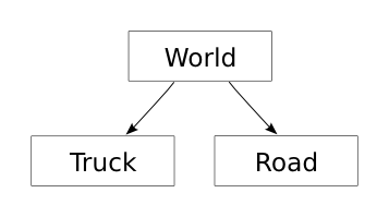
Figure 1.1: A scene graph for a scene consisting of a road and a truck.
It turns out that there is a great chance that if you render this scene just like it is, the truck will appear floating in the air, or buried into the ground, or in any other place different than the one you intended. You’ll have to translate it to its right position. Fortunately, doing that is fairly simple, because some nodes of the scene graph can be used to represent this kind of transform. Therefore, to fix the truck position, you just have to add a node representing a translation, yielding the scene graph shown on Figure 1.2.
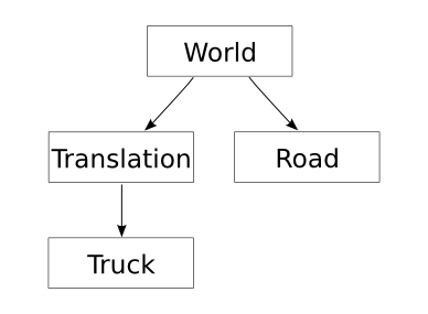
Figure 1.2: A scene graph for a scene consisting of a road and a translated truck.
The hierarchical structure of the scene graph lends itself to some neat features. Let’s suppose that we want to add two crates to the scene. The first one will be on the road, and the second one will be loaded on the truck. For the same reason as before, we’ll add a translation node above the nodes representing the crates. The graph for this scene is shown in Figure 1.3.
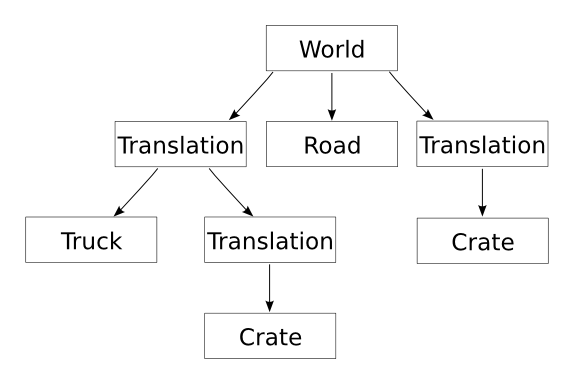
Figure 1.3: A scene graph for a scene consisting of a road, a truck and two crates.
The neat thing about this is that a translation node affects whatever is below it on the graph, even other translation nodes. In this case, notice that there are two translations between the crate on the truck and the root of the graph. The first of these translations (the one closest to the root) affects both the truck and the crate, that is, if we change it, the truck will be moved and the crate loaded on it will be moved along with it. On the other hand, if we change the second translation (the one immediately above the crate), only the crate will be moved. In other words, this scene graph allows us to easily position both the crate inside the truck and the “bundle” of the truck and the crate at the same time. As you see, the structure matches the semantics of the real scene pretty well.
By now, you are possibly wondering why scene graphs are called a graphs if they all look like trees. Well, the examples so far were trees, but that is not always the case. In our last graph, we had two crates. Since both crates look exactly the same, you don’t have to create a node for each one of them. One node “referenced” twice does the trick, as Figure 1.4 illustrates. During rendering, the “Crate” node will be visited (and rendered) twice, but some memory is spared because the model is loaded just once.
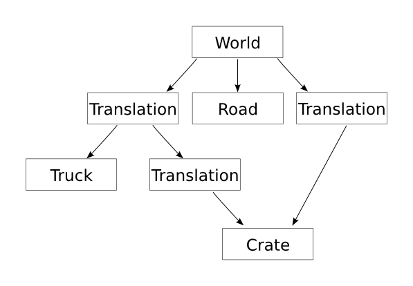
Figure 1.4: A scene graph for a scene consisting of a road, a truck and a pair of crates — with a single node for the two crates.
We could have used a single node for the two (or more than two) crates even if they didn’t look exactly the same. We could have added a “scale” node in one of the two paths leading to the crate node, for instance. That way, one crate would look larger than the other. We could also do some tricks to make one of the crates of a different color, or in wireframe, or translucent… but these are topics for the next part of this series.
Anyway, as you can see, scene graphs can get more complicated than what I have shown so far, but the simple notion just presented shall be enough for a while. The thing to keep is mind is that, in general, geometry intended to be rendered will be at the leaf nodes; the non-leaf nodes will establish a hierarchy among the scene elements and perform some tricks like geometric transformations.
And now, it’s time to say a couple more words concerning a second fundamental question.
The question is: “who cares?”
Anyone wanting performance cares. The scene graph structure allows to implement with some ease several optimization techniques. To begin with, its hierarchical structure naturally leads to a spatially subdivided scene, which lends to frustum culling (objects not in the field of view are not even sent to the graphics pipeline). Level-of-detail techniques can be implemented in a special node type that handles all the dirty details. It also makes easier to minimize changes to the rendering state (see “Part 2”), which is yet another way to make your software perform better.
Anyone wanting productivity cares. If you write a nontrivial 3D application, you will definitely need a well-though data structure to organize your scene, otherwise you will spend more time fighting with your code than writing features that will make your users happy. Scene graphs are one of such data structures, possibly the most widely used one. Many real programs, running today in many different areas rely on scene graphs. Scene graphs provide a clean and extensible foundation for 3D software. You may need some time to learn them, but on the long run this time investment pays off.
Anyone wanting scalability cares. Scene graphs make it easier to create applications that run in a wide range of hardware, from small devices (the kind of thing normal people carry on their pockets) to large and expensive multi-pipeline graphics systems (the kind of thing normal people don’t have at home).
These are all potential advantages of any scene graph. The Open Scene Graph, in particular, is pretty good in what regards performance, productivity and scalability. Furthermore, OSG has lots of features commonly needed in 3D applications, like loaders for 2D images and 3D models, routines for testing for intersections and paging large 3D data sets from disk, which further increase the productivity. Hence, if you are developing 3D applications, you should care, too.
Something OSG-related, at last
Up to this point, the discussion was around “generic” scene graphs. From now on,
all examples will use exclusively OSG scene graphs, that is, instead of using a
generic “Translation” node, we’ll be using an instance of a real class defined
in the OSG node hierarchy. A node in OSG is represented by the osg::Node
class. Although technically possible, there is not much use in instantiating
osg::Nodes; things start to get interesting when we look at some of its
subclasses. In this chapter, three of these subclasses will be introduced:
osg::Geode, osg::Group and osg::PositionAttitudeTransform. We’ll
also see one OSG fundamental class that is not a node: osg::Drawable.
The osg::Drawable class is the ultimate source of renderable stuff. Of course,
you can can think of the whole scene graph (or subset of it, for that matter) as
being renderable, but the real renderable data, the real vertices and
polygons, reside ultimately in an osg::Drawable.
However, as I said above, osg::Drawables are not nodes, so we cannot attach
them directly to a scene graph. It is necessary to use a “geometry node”,
osg::Geode, instead. Hence, our scene graphs must have one (or more)
osg::Drawables with the real geometry, and it must be attached to one (or
more) osg::Geode, so that the geometry can end up in the scene graph.
Not every node in an OSG scene graph can have other nodes attached to them as
children. In fact, we can only add children to nodes that are instances of
osg::Group or one of its many subclasses.
Using osg::Geodes and an osg::Group, it is possible to recreate the scene
graph from Figure 1.1 using real classes from OSG. The result is shown in Figure
1.5.
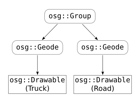
Figure 1.5: An OSG scene graph, for the same scene of Figure 1.1. Instances of OSG classes derived from osg::Node are drawn in rounded boxes with the class name inside it. osg::Drawables are represented as rectangles.
That’s not the only way to convert the scene graph from Figure 1.1 to a real OSG
scene graph. Since more than one osg::Drawable can be attached to a single
osg::Geode, the scene graph shown in Figure 1.6 is also an OSG version of
Figure 1.1.
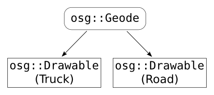
Figure 1.6: An alternative OSG scene graph representing the same scene as the one in Figure 1.5.
The scene graphs of Figures 1.5 and 1.6 have the same problem as the one in the
Figure 1.1: the truck will probably be at the wrong position. And the solution
is the same as before: translating the truck. In OSG, probably the simplest way
to translate a node is by adding an osg::PositionAttitudeTransform node above
it. An osg::PositionAttitudeTransform has associated to it not only a
translation, but also an attitude (orientation, or rotation) and a scale.
Although not exactly the same thing, this can be though as the OSG equivalent to
the OpenGL calls glTranslate(), glRotate() and glScale(). Figure 1.7 is
the OSGfied version of Figure 1.2.
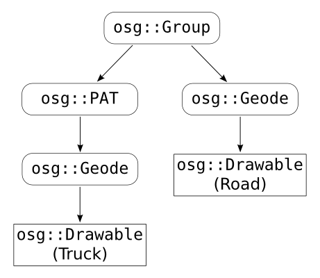
Figure 1.7: An OSG scene graph, for the same scene of Figure 1.2. For compactness, osg::PositionAttitudeTransform is written as osg::PAT.
For completeness, Figures 1.8 and 1.9 show the OSG way to represent the “generic” scene graphs from Figures 1.3 and 1.4.
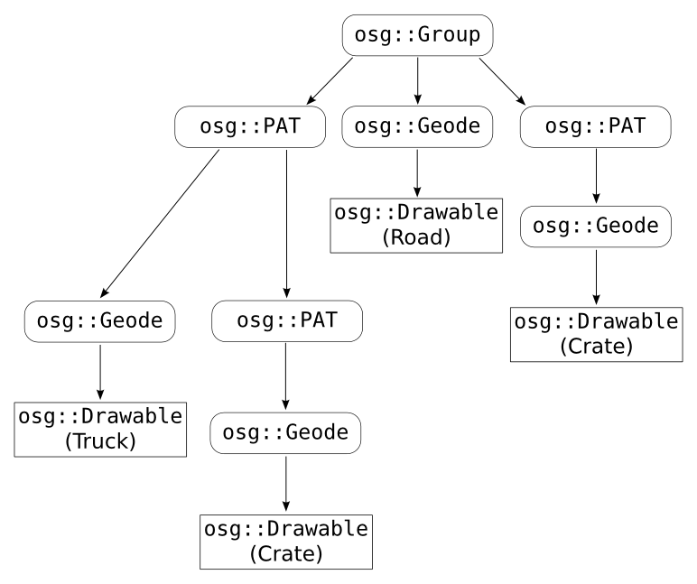
Figure 1.8: An OSG scene graph equivalent to the generic scene graph of Figure 1.3.
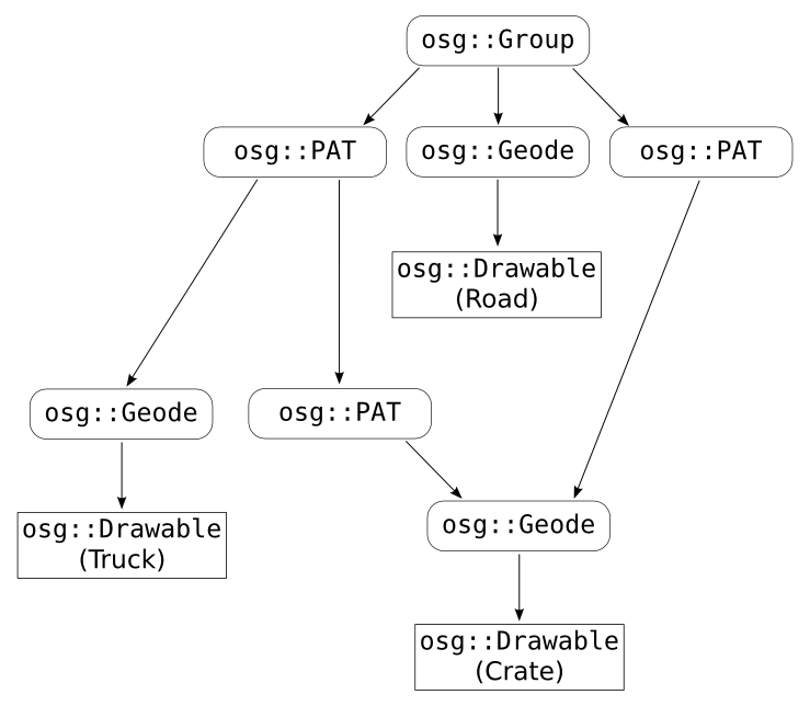
Figure 1.9: An OSG scene graph equivalent to the generic scene graph of Figure 1.4.
Smart pointers and OSG
Save the whales. Feed the hungry. Free the mallocs.
— fortune(6)
Sadly, it looks like quite a few C++ users are unfortunate enough to not be proficient with smart pointers. Since OSG uses smart pointers extensively (as every C++ program should.), it seems worthwhile to spend some time explaining them. Don’t dare to skip this section if “smart pointers” sounds like Greek for you (and you are not Greek, that’s it).
Let’s start with a definition: a resource is anything that must be allocated
before being used and deallocated when no longer needed. Perhaps the most common
resource we use when programming is heap memory, but many other examples exist.
Two common cases are files (which must be closed after being opened) and
database transactions (which have to be committed or rolled back after being
“beginned”). Also in OpenGL there are some examples of resources (one example
are texture names generated by glGenTextures() which must be freed by
glDeleteTextures()).
The most fascinating thing related to resources is the fact that there exist so many programmers who believe that they can handwrite code capable of freeing them in every case and will never forget to write such code. This thinking only leads to resource leaks. The good news is that, with some discipline, this freeing task can be passed to the C++ compiler, which is much more reliable than us for tasks like this.
The main ideas behind resource management in C++ are worth of mentioning here, but complete discussion about this is beyond the scope of this text.1 Speaking of “scope”, the scope of “automatic” variables (that is, variables allocated on the stack) plays a central role in resource management in C++: the language rules guarantee that the destructor of an object allocated on the stack will be called when it gets out of scope. How does this help to avoid resource leaks? Take a look at the following class:
class ThingWrapper
{
   public:
      ThingWrapper()
      {
         handle_ = AllocateThing();
      }

      ~ThingWrapper()
      {
         DeallocateThing(handle_);
      }

      ThingHandle& get()
      {
         return handle_;
      }

   private:
      ThingHandle handle_;
};
It allocates a Thing in the constructor and frees it in the destructor. So,
whenever we need a Thing we can do something like this:
ThingWrapper thing;
UseThing(thing.get());
Instantiating a ThingWrapper allocates a Thing (in ThingWrapper’s
constructor). But the nice part is that the Thing will be automatically freed
when thing gets out of scope, since its destructor is guaranteed to execute
when this happens. Voilà. Automatic resource management.
The class ThingWrapper is an example of a C++ programming technique usually
called “resource acquisition is initialization” (RAII). A smart pointer is
simply a class (or, more commonly, a class template) that uses the RAII
technique to automatically manage heap memory. Quite like ThingWrapper, but
instead of calling hypothetical AllocateThing() and DeallocateThing()
functions, a smart pointer typically receives a pointer to newly allocated
memory in its constructor and uses the C++ operator delete to free that memory
in the destructor.
In the ThingWrapper example, thing is said to be owner of the Thing
allocated with AllocateThing(), and therefore is responsible for deallocating
it. With scene graphs, there is an extra detail to complicate the things a
little bit: sometimes an object has more than one owner. For example, in the
scene graph shown in Figure 1.9, the osg::Geode with the crate attached to it
has two parents. Which one should be responsible for freeing it?
In these cases, the resource shall not be deallocated while there is at least
one reference pointing to it. Most objects in OSG have an internal counter with
the number of references pointing to it. (To be more exact, the OSG objects with
an embedded reference count are all those that are instances of classes derived
from osg::Referenced.) The resource (that is, the object) will only be
destroyed when its internal reference count goes down to zero.
Fortunately, we programmers are not expected to manage these reference counts
manually: that’s why smart pointers exist for. In OSG, smart pointers are
implemented as a class template named osg::ref_ptr<>. Whenever an OSG object
receives a pointer to another OSG object, it is immediately stored in an
osg::ref_ptr<>. This way, the reference count of the underlying object is
automatically managed, and the object will be automatically deallocated when it
is no longer being referenced by anyone.
The example below shows OSG’s smart pointers in action. The example is followed by some notes about it.
// SmartPointers.cpp

#include <cstdlib>
#include <iostream>
#include <osg/Geode>
#include <osg/Group>

void MayThrow()
{
   if (rand() % 2)
      throw "Aaaargh!";
}

int main()
{
   try
   {
      srand(time(0));
      osg::ref_ptr<osg::Group> group (new osg::Group());

      // (1) This is OK, albeit a little verbose.
      osg::ref_ptr<osg::Geode> aGeode (new osg::Geode());
      MayThrow();
      group->addChild (aGeode);

      // (2) This is quite safe, too.
      group->addChild (new osg::Geode());

      // (3) This is dangerous! Don't do this!
      osg::Geode* anotherGeode = new osg::Geode();
      MayThrow();
      group->addChild (anotherGeode);

      // Say goodbye
      std::cout << "Oh, fortunate one. No exceptions, no leaks.\n";
   }
   catch (...)
   {
      std::cerr << "'anotherGeode' possibly leaked!\n";
   }
}
Concerning the example above, the first thing to notice is that it gives a first and rough idea on how to “compose” scene graphs like the ones depicted in the figures shown before (this is just for the curiosity sake; we’ll address this properly soon). The real intent of this example is showing two safe ways of using OSG’s smart pointers and one dangerous way to not use them.
The section marked as (1), shows one safe way to use the smart pointers:
Initially, an osg::ref_ptr<> (called aGeode) is explicitly created and
initialized with a newly allocated osg::Geode (the resource). At this point,
the reference count of the geode allocated on the heap equals to one (since
there is just one osg::ref_ptr<>, namely aGeode, pointing to it.) Two lines
latter, the geode is added as a child of a group. As soon as this happens, the
group increments the geode’s reference to two. Now, what if something bad
happens? What if the call to MayThrow() actually throws? Well, aGeode will
get out of scope and will be destroyed. Its destructor will decrement the
geode’s reference count. And, since it was decremented to zero, it will also
properly dispose the geode. There is no memory leak.
The next section, maked as (2), does more or less the same thing as the previous
case. The difference is that the geode is allocated with operator new and
added as group’s child in a single line of code. This is quite safe, too,
because there are not many bad things that can happen in between (after all,
there is nothing in between.)
The bad, wrong, dangerous, flawed and condemnable way to manage memory is shown
in section (3). It looks like the first case, but anotherGeode is allocated
with new and stored in a “dumb” pointer (a regular C++ pointer). If
MayThrow() throws, nobody will call delete on the geode and it will leak.
There is another thing that can be said here: osg::Referenced’s destructor
isn’t even public, so you are not able to say delete anotherGeode. Instances
of classes derived from osg::Referenced (like osg::Geode) are simply meant
to be managed automatically by using osg::ref_ ptr<>s. So, do the right thing
and never write code like in this third case. The world will be a better place.
Time to show something on the screen
I would feel guilty to end this first part without at least a single example program that actually shows something on the screen. This program is a very simple 3D viewer; basically, all it does is loading the file passed as a command-line parameter and displaying it on the screen. So, without further delays, here is its source code.
// VerySimpleViewer.cpp

#include <iostream>
#include <osgDB/ReadFile>
#include <osgViewer/Viewer>

int main(int argc, char* argv[])
{
   // Check command-line parameters
   if (argc != 2)
   {
      std::cerr << "Usage: " << argv[0] << " <model file>\n";
      exit(1);
   }

   // Load the model
   osg::ref_ptr<osg::Node> loadedModel = osgDB::readNodeFile(argv[1]); // (1)

   if (!loadedModel)
   {
      std::cerr << "Problem opening '" << argv[1] << "'\n";
      exit(1);
   }

   // Create a viewer, use it to view the model
   osgViewer::Viewer viewer;
   viewer.setSceneData(loadedModel); // (2)

   // Enter rendering loop
   viewer.run(); // (3)
}
This example is pretty simple, but there are one or two things that can be said
about it. To begin with, OSG knows how to read several formats of 3D models and
images, and all the functions and classes related to this are declared in the
namespace osgDB. The line marked with (1) uses one of such functions,
osgDB::readNodeFile(), which takes as parameter the name of a file containing
a 3D model and returns a pointer to an osg::Node. The returned node contains
all information necessary to render the 3D properly, including, for example,
vertices, polygons, normals and texture maps. As you may guess, it possibly is a
complex scene graph on its own right, with several groups, nodes, drawables and
more. But this is all beautifully hidden behind a single call to
osgDB::readNodeFile() and its single returned osg::Node.
Also notice how we actually get our scene graph displayed by attaching it to an
osgViewer::Viewer object (the call to setSceneData(), (2)) and starting
the viewer (the call to run(), (3)). After that point, our program will
run forever (or until the user presses ESC, whatever comes first). I must note
that we are not strictly required to use an osgViewer::Viewer, but that’s the
easiest way to go, and the alternatives don’t belong to a very introductory
guide like this one.
Ready for more OSG? Part 2 is here.
-
There is a nice introduction to resource management at Reliable Software’s website. The latest revision of the C++ programming language includes smart pointers modeled after the ones provided by Boost; so, checking out their documentation may be a good idea, too. ↩︎